Matrix Optics
![]()
![]()
Introduction
The optical beam passing through the interface of different refractive indices, changes its direction towards/away normal to the interface, and the changed direction can be calculated mathematically using refractive indices making that interface. To understand this, we can consider an example illustrated in Figure 1. Assuming $n_2$ to be sand. If a car enters into a region with higher refractive index at oblique angle, its right front wheel enters into an area of $n_2$ earlier than the left front wheel, hence starts facing lossy force earlier, causing a change in direction towards the normal. Same intuition can help to predict diverted optical path of optical beam.
But if a linearly polarized light faces an interface of higher refractive index it gets refracted and reflected. The direction of beam propagation ($\vec {k}$) is shown in figure 2 and sinusoidal waves shows that the oscillation of electric field is perpendicular to the direction of wave propagation. Optical beam is characterized as $p$–polarized, if electric field oscillations are perpendicular to the plane formed by incident, reflected and transmitted beam, and $p$ if oscillations are in the same plane. The direction of reflected and transmitted beams can be calculated by using Snell’s Law and intensities can be computed via Fresnel coefficients as:
\[\begin{aligned} r_p &= \frac{n_2\cos\theta_1-n_1\cos\theta_2}{n_2\cos\theta_1+n_1\cos\theta_2}, (1) \\ r_s &= \frac{n_1\cos\theta_1-n_2\cos\theta_2}{n_1\cos\theta_1+n_2\cos\theta_2}, (2) \\ t_p &= \frac{2 n_1\cos\theta_1}{n_2\cos\theta_1+n_1\cos\theta_2}, (3) \\ r_s &= \frac{2 n_1\cos\theta_1}{n_1\cos\theta_1+n_2\cos\theta_2}. (4) \end{aligned}\]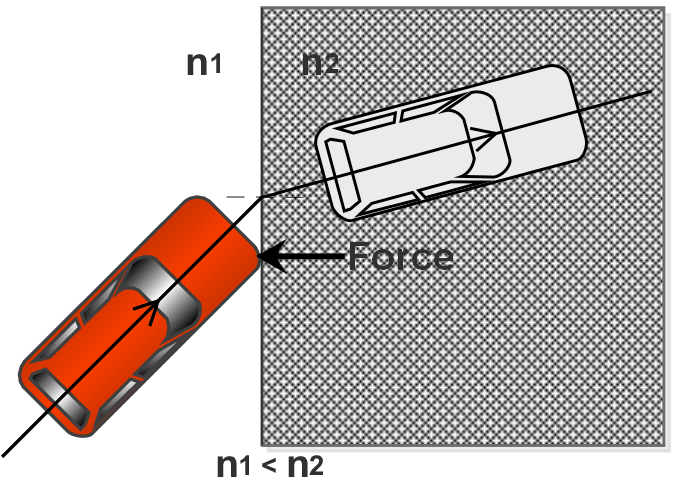
Figure 1: Car entering into sand (intuition)
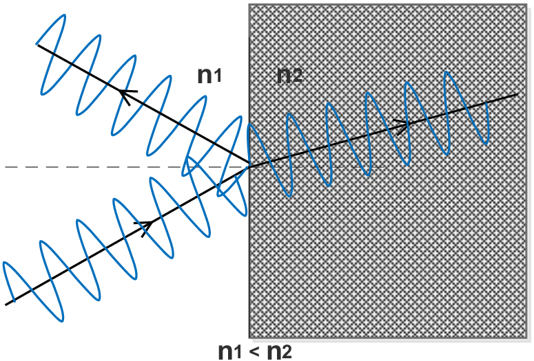
Figure 2: Refraction of optical beam at the interface between two media of different refractive indices
These coefficients can easily be used on single interface, but for multilayered system, matrix transformation method is more useful.
Matrix Method
Suppose we have a multilayered system[@zangwill_zangwill_2018] having $N$ refractive indices stacked together making $N-1$ interfaces with refractive index $n_j$, impedance $Z_j$, thickness $d_j$ for layer $j$. Also the layer $0$ is semi–infinite with $Z = - \infty$ and layer $N$ is being treated semi–infinite with $Z = \infty$ and phase change is $\phi_j$.
\[\begin{aligned} \begin{bmatrix} E_{j-1} \\\\ H_{j-1}\end{bmatrix} &= \begin{bmatrix} \cos \phi_j & i\sin \phi_j / Z_j \\\\ Z_j i\sin \phi_j & \sin \phi_j \end{bmatrix} \begin{bmatrix} E_{j} \\\\ H_{j}\end{bmatrix} (5) \end{aligned}\]Eq. 5 relates amplitudes in one layer to the next adjacent layer and therefore repeated application of transfer matrix allows us to propagate waves from one side of the multilayer system to the other using
\[\begin{aligned} \begin{bmatrix} E_{1} \\\\ H_{1})\end{bmatrix} &= \prod_{j=2}^{N-1} \begin{bmatrix} \cos \phi_j & i\sin \phi_j / Z_j \\\\ Z_j i\sin \phi_j & \sin \phi_j)\end{bmatrix} \begin{bmatrix} E_{N} \\\\ H_{N}\end{bmatrix} (6) \end{aligned}\]And the characteristic matrix for the entire system will be
\[\begin{aligned} M= \begin{bmatrix} m_{11} & m_{12} \\\\ m_{21} & m_{22}\end{bmatrix} &= \prod_{j=1}^{N-1} \begin{bmatrix} \cos \phi_j & i\sin \phi_j / Z_j \\\\ Z_j i\sin \phi_j & \sin \phi_j \end{bmatrix}. (7) \end{aligned}\]Here, $Z_j = \sqrt{\frac{\epsilon_0}{\mu_0}}n_j\cos\theta_j$ and by applying the boundary conditions for Figure 3, we have
\[\begin{aligned} Z_0 = \sqrt{\frac{\epsilon_0}{\mu_0}}n_0\cos\theta_i \quad\text{and}\quad Z_N = \sqrt{\frac{\epsilon_0}{\mu_0}}n_N\cos\theta_t. \end{aligned} (8)\]Consequently,
\[\begin{aligned} r &= \frac{Z_{1} m_{11} + Z_{1} Z_{N} m_{12} - m_{21} - Z_{N}m_{22}}{Z_{1} m_{11} + Z_{1} Z_{N} m_{12} + m_{21} + Z_{N}m_{22}} (9)\\ t &= \frac{2Z_{1}}{Z_{1} m_{11} + Z_{1} Z_{N} m_{12} + m_{21} + Z_{N}m_{22}} (10) \end{aligned}\]To find $r$ or $t$ for any configuration of multilayered system, we only need to compute the characteristic matrices for each film, multiply them and substitute resulting matrix elements into the Eqs. 9 and 10).
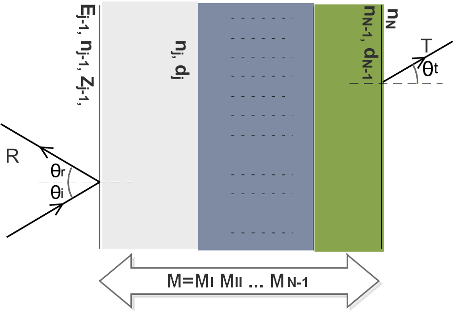
Fig 3: Propagation of optical beam through a multilayer structure consisting of the materials with different indices of refraction.
To find reflection and transmission coefficients, we have
\(\begin{aligned} R = rr' \quad\text{and}\quad T = tt', (11) \end{aligned}\) where $r’$ and $t’$ are the complex conjugates of $r$ and $t$.
Algorithm
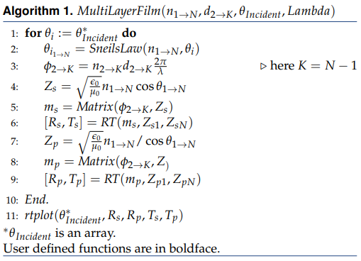
We implement the matrix transformation method via MATLAB. Syntax of such function is
\[[\theta_\text{incident},R_s,R_p,T_s,T_p]=\textit{MultiLayerFilm}(n_{1 \rightarrow N},d_{2 \rightarrow K},\theta_\text{incident},\lambda)\]Here MultiLayerFilm is the MATLAB function whose algorithm is shown in algorithm (1),
Let we have two layers of thickness 1 mm and 0.2 mm separated with distance of 0.3 mm having refractive indices $1.4, 1.5$, wavelength 1547 nm. Now we want to find $R_s, R_p, T_s, T_p$ for incident angles from to with the following function.
% n (Glass) = 1.47
% n (Borosilicate Glass) = 1.5007
% d (Glass) = 1mm
% d (Air) = 0.302 mm
% d (Borosilicate Glass) = 2.228 mm
[Incident,RS,RP,TS,TP] = ...
MultiLayerFilm([1 1.47 1.5007 1],[1e-3 0.302e-3 2.228e-3],0:90,1547e-9)
This generate arrays Incident, RS, RP, TS, TP corresponding to
$\theta_\text{incident}, R_s, R_p, T_s, T_p$, as shown in
figure 4{reference-type=”ref” reference=”fig:4”}
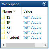
Figure 4: Workspace of MATLAB showing output values of function MultiLayerFilm
Experimental Setup
Experimental setup is shown in Figure 7. We used two transparent materials of thickness 1 mm, 2.288 mm having refractive indices $1.47, 1.5007$ (at $\lambda = 1547 nm$) with separation of 0.302 mm and placed on a rotating table. Optical power sensor that can be rotated along the table to measure transmitted/reflected beam. Actual setup is shown in Figure 6 and measured reflection and transmission coefficients for $\theta_i \text{from } {1} \text{ to } {90}$ and measured corresponding transmission and reflection power amplitudes, for both $s$ and $p$ polarized optical beams.
Results and Discussion
Figure 5 show results of our experimentally measured transmission/reflection intensities, measured for different incident angles $\theta_i({0} \rightarrow {90})$. Here lines represent theoretical plots generated by algorithm 1 and stars represent experimental measurements which exactly matches to the observations based on MATLAB algorithm.
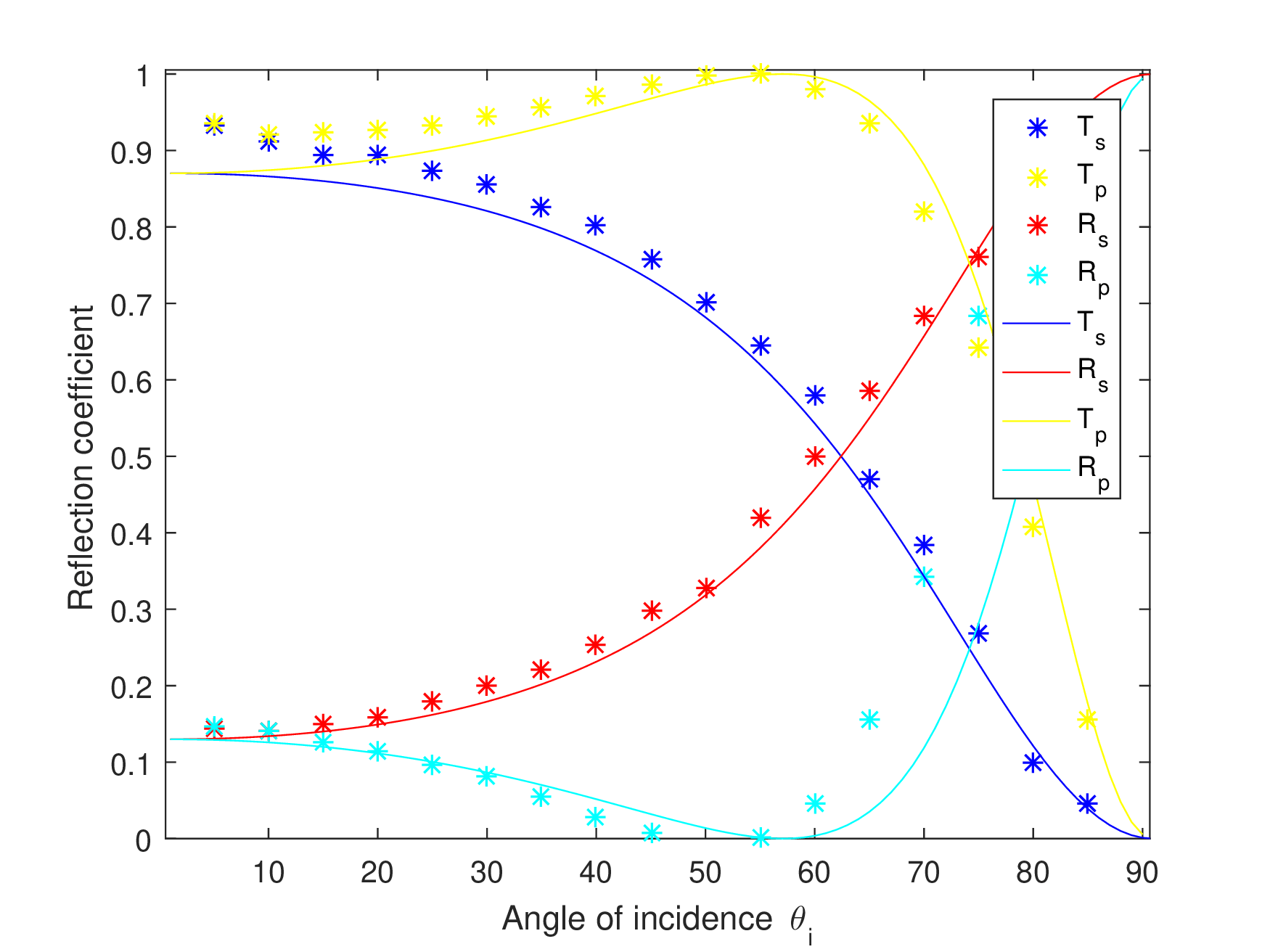
Figure 5: Power coefficients, lines show theoretical and stars show experimental results.
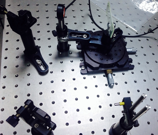
Figure 6: Screen shot of experimental setup
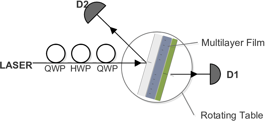
Figure 7: Schematic diagram of experimental setup.